Algorithm

Data Sets

Blood samples were collected from a total of 1037 unrelated animals belonging to twenty two different Indian goat breeds viz. Blackbengal, Ganjam, Gohilwari, Jharkhandblack, Attapaddy, Changthangi, Kutchi, Mehsana, Sirohi, Malabari, Jamunapari, Jhakarana, Surti, Gaddi, Marwari, Barbari, Beetal, Kanniadu, Sangamnari, Osmanabadi, Zalawari and Cheghu across India, over 10 years. The breeds selected were from diverse geographical regions and climatic conditions with varying utilities and body sizes. Genomic DNA was isolated from the blood samples by using SDS-Proteinase-K method. The quality and quantity of the DNA extracted was assessed by Nanodrop 1000 (Thermo Scientific, USA) before further use. 55000 allelic data of microsatellite marker based DNA fingerprinting of 22 goat breeds. These data are on 25 loci viz. ILST008, ILSTS059, ETH225, ILSTS044, ILSTS002, OarFCB304, OarFCB48, OarHH64, OarJMP29, ILSTS005, ILSTS019, OMHC1, ILSTS087, ILSTS30, ILSTS34, ILSTS033, ILSTS049, ILSTS065, ILSTS058, ILSTS029, RM088, ILSTS022, OarAE129, ILSTS082 and RM4 (Table 1). The system had been trained for 55000 microsatellite data on 25 loci to achieve the best fitted model for breed identification.

Table 1. List of 25 loci along with the primer pairs

Locus	Forward Primer	Reverse Primer	Dye	Size Range
ILST008	gaatcatggattttctgggg	tagcagtgagtgaggttggc	FAM	167-195
ILSTS059	gctgaacaatgtgatatgttcagg	gggacaatactgtcttagatgctgc	FAM	105-135
ETH225	gatcaccttgccactatttcct	acatgacagccaagctgctact	VIC	146-160
ILST044	agtcacccaaaagtaactgg	acatgttgtattccaagtgc	NED	145-177
ILSTS002	tctatacacatgtgctgtgc	cttaggggtgtattccaagtgc	VIC	113-135
OarFCB304	ccctaggagctttcaataaagaatcgg	cgctgctgtcaactgggtcaggg	FAM	119-169
OarFCB48	gagttagtacaaggatgacaagaggcac	gactctagaggatcgcaaagaaccag	VIC	149-181
OarHH64	cgttccctcactatggaaagttatatatgc	cactctattgtaagaatttgaatgagagc	PET	120-138
OarJMP29	gtatacacgtggacaccgctttgtac	gaagtggcaagattcagaggggaag	NED	120-140
ILSTS005	ggaagcaatgaaatctatagcc	tgttctgtgagtttgtaagc	VIC	174-190
ILSTS019	aagggacctcatgtagaagc	acttttggaccctgtagtgc	FAM	142-162
OMHC1	atctggtgggctacagtccatg	gcaatgctttctaaattctgaggaa	NED	179-209
ILSTS087	agcagacatgatgactcagc	ctgcctcttttcttgagagc	NED	142-164
ILSTS30	ctgcagttctgcatatgtgg	cttagacaacaggggtttgg	FAM	159-179
ILSTS34	aagggtctaagtccactggc	gacctggtttagcagagagc	VIC	153-185
ILSTS033	tattagagtggctcagtgcc	atgcagacagttttagaggg	PET	151-187
ILSTS049	caattttcttgtctctcccc	gctgaatcttgtcaaacagg	NED	160-184
ILSTS065	gctgcaaagagttgaacacc	aactattacaggaggctccc	PET	105-135
ILSTSO58	gccttactaccatttccagc	catcctgactttggctgtgg	PET	136-188
ILSTSO29	tgttttgatggaacacagcc	tggatttagaccagggttgg	PET	148-191
RM088	gatcctcttctgggaaaaagagac	cctgttgaagtgaaccttcagaa	FAM	109-147
ILSTS022	agtctgaaggcctgagaacc	cttacagtccttggggttgc	PET	186-202
OARE129	aatccagtgtgtgaaagactaatccag	gtagatcaagatatagaatatttttcaacacc	FAM	130-175
ILSTS082	ttcgttcctcatagtgctgg	agaggattacaccaatcacc	PET	100-136
RM4	cagcaaaatatcagcaaacct	ccacctgggaaggccttta	NED	104-127

Input/ Submission
STR alleles can be submitted directly in numerical values of base pair. Goat being diploid thus needs submission of both alleles of homologous chromosome. Alternatively the submission can also be done in a single file with format .txt or .csv and 50 records.

Machine Learning Workbench Used
WEKA machine learning workbench, (developed by The University of Waikato), with extensive collection of machine learning algorithms and data pre-processing methods was used for classification and prediction. A suitable algorithm for generating an accurate predictive model was identified from it.
This is available at http://www.cs.waikato.ac.nz/ml/weka.

Bayesian Network as Classifier
Classification is a technique to identify class labels for instances based on a set of features (attributes). Application of BNs techniques to classification involves BN learning (training) and BN inference to classify instances. It has powerful probabilistic representation for classification and has received considerable attention in the recent past.
A Bayesian network B may be induced and encodes a probability distribution   from a given training set. The resulting model can be used so that given a set of attributes , the classifier based on B returns the label c which maximizes the posterior probability, i.e.  
Let  denotes the training data set. Here, each  is a tuple of the form which assigns values to the attributes  and to the class variable C. The log likelihood function, which measures the quality of learned model can be written as

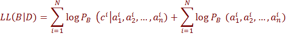
The first term in this equation measures efficiency of B toestimates the probability of a class given set of attribute values. The second term measures how well B estimates the joint distribution of the attributes. Since the classification is determined based on 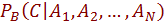, only the first term is related to the score of the network as a classifier i.e., its predictive accuracy. This term is dominated by the second term, when there are many observations. As n grows larger, the probability of each particular assignment to  becomes smaller, since the number of possible assignments grows exponentially in n.

Cross Validation
Five-fold cross validation technique was implemented, where the data sets were randomly divided into five equal sets and each set containing almost equal number of observations. These sets were grouped into training and test set.  Among these, four sets were used for training and the remaining one set for testing. The process was repeated five times such that each set gets the opportunity to fall under testing. Average of five sets is calculated finally.

Assessment of Prediction Accuracy
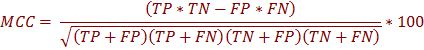
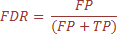
Computational models that are valid, relevant, and properly assessed for accuracy can be used for planning of complementary laboratory experiments. The prediction quality was examined by testing the model, obtained after training the system, with test data set. Several measures are available for the statistical estimation of the accuracy of prediction models. The common statistical measures are Sensitivity, Specificity, Precision or Positive predictive value (PPV), Negative predictive value (NPV), False Discovery Rate (FDR), Accuracy and Mathew’s correlation coefficient (MCC).

The Sensitivity indicates the ‘‘quantity’’ of predictions, i.e., the proportion of real positives correctly predicted. The Specificity indicates the ‘‘quality’’ of predictions, i.e., the proportion of true negatives correctly predicted. The PPV indicates the proportion of true positives in predicted positives-“the success rate” while NPV is the proportion of true negatives in predicted negatives.

These measures are defined as follows:

Where

TP = True Positive : are defined as the correctly identified instances
TN = True Negative : are defined as the correctly rejected instances
FP = False Positive : are defined as the incorrectly identified instances
FN = False Negative : are defined as the incorrectly rejected instances